Image retrieval app using Apple’s 4M-21 any-to-any vision model

1 Image retrieval App

Figure 1: Image retrieval using 4M-21 any-to-any vision model

Before, we get started, let’s take a moment to understand what’s going on in the demo video above:

1. This a demo of an image retrieval app that is capable of retrieving most similar images from any given database. It is built on top of gradio.
2. As part of this demo, we are able to retrieve images based on the following filters:
   1. Caption (description of the image)
   2. Brightness (brightness in the image, lower represents a darker image)
   3. Number of items (lower represents fewer number of items in the image)
3. Starting with a 5/255 brightness & a 5/50 items per image for dining room, we were able to retrieve an almost empty & dark image of a dining room.
4. Increasing the number of items to 50 retrieves a dark image of a dining room but with chairs and a dining table.
5. As you’ll later see, we can also add a lot more filters such as an input image, image segmentation mask, image boundary, number of humans and more but we have limited ourselves to three for the purpose of this demo.

With this understanding of the demo app, let’s get started and build one ourselves! If you’d like to skip over all the details, python code for this app has been shared in Section 2.3.

Note

Thank you jarvislabs.ai for the compute, this blog post would not have been possible without the credits.

1.1 Prerequisites

As part of this blog post, we are going to assume that the reader has a basic understanding of embeddings, Vision Language Models and image retreival using cosine similarity search.

Some good resources to get the readers going are shared below:

1. Image Similarity with Hugging Face Datasets and Transformers by Sayak Paul
2. The illustrated word2vec by Jay Alammar
3. Vision Language Models Explained by Merve Noyan & Edward Beeching

2 4M-21: An Any-to-Any Vision Model for Tens of Tasks and Modalities

2.1 Introduction

As part of this blog post we will be utilising Apple’s 4M-21: An Any-to-Any Vision Model for Tens of Tasks and Modalities Bachmann et al. (2024) paper to build a real-time search engine that is capable of using caption, brightness & number of items per image as filters to query an image database of a total of 15 images. Though this technique can easily be expanded to a million or more images. If you have a big database of images, take a look at faiss for similarity search.

We will build an app using Gradio and also deploy it to Huggingface Hub for anyone to use.

The 4M-21 paper is the second in the 4M series (Massively Multimodal Masked Modeling) by Apple, the first paper was also an any-to-any vision model capable of working with 7 modalities - 4M: Massively Multimodal Masked Modeling Mizrahi et al. (2023).

Figure 2: 4M-21 any-to-any vision model

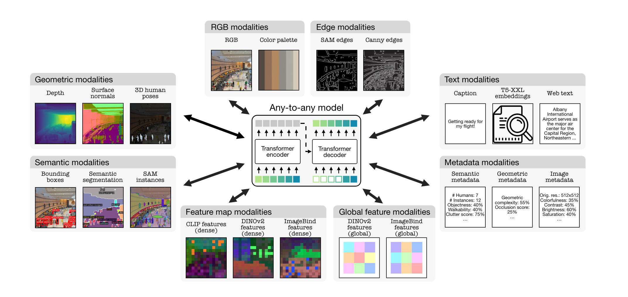
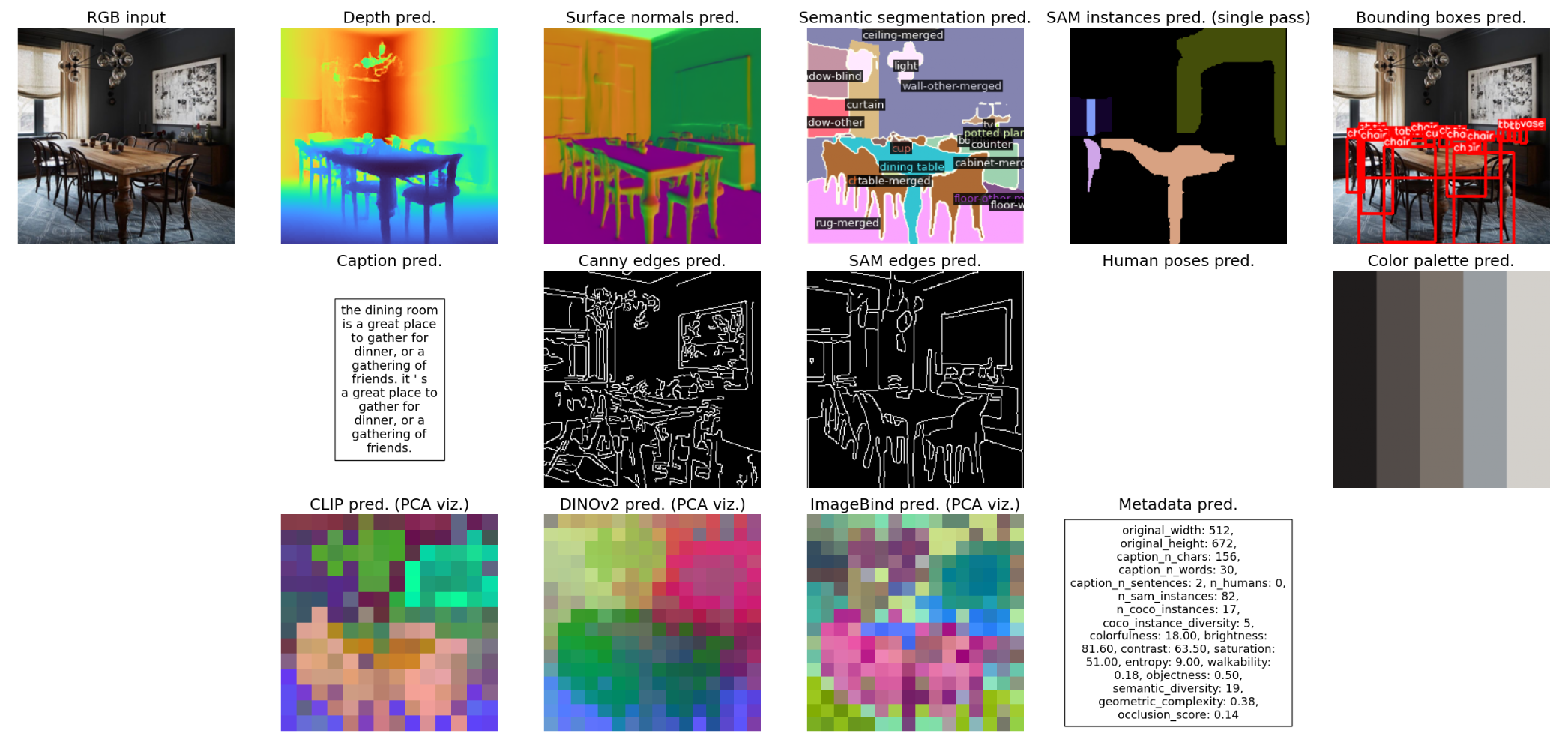
As shown in the image above, the model can work with with multiple modalities. It can take all modalities as inputs and output any or all of the modalities using single or subset of modalities! Unbelievable right? Not anymore!

See the conditional generation example below as shared in the paper:

Figure 3: One to all generation

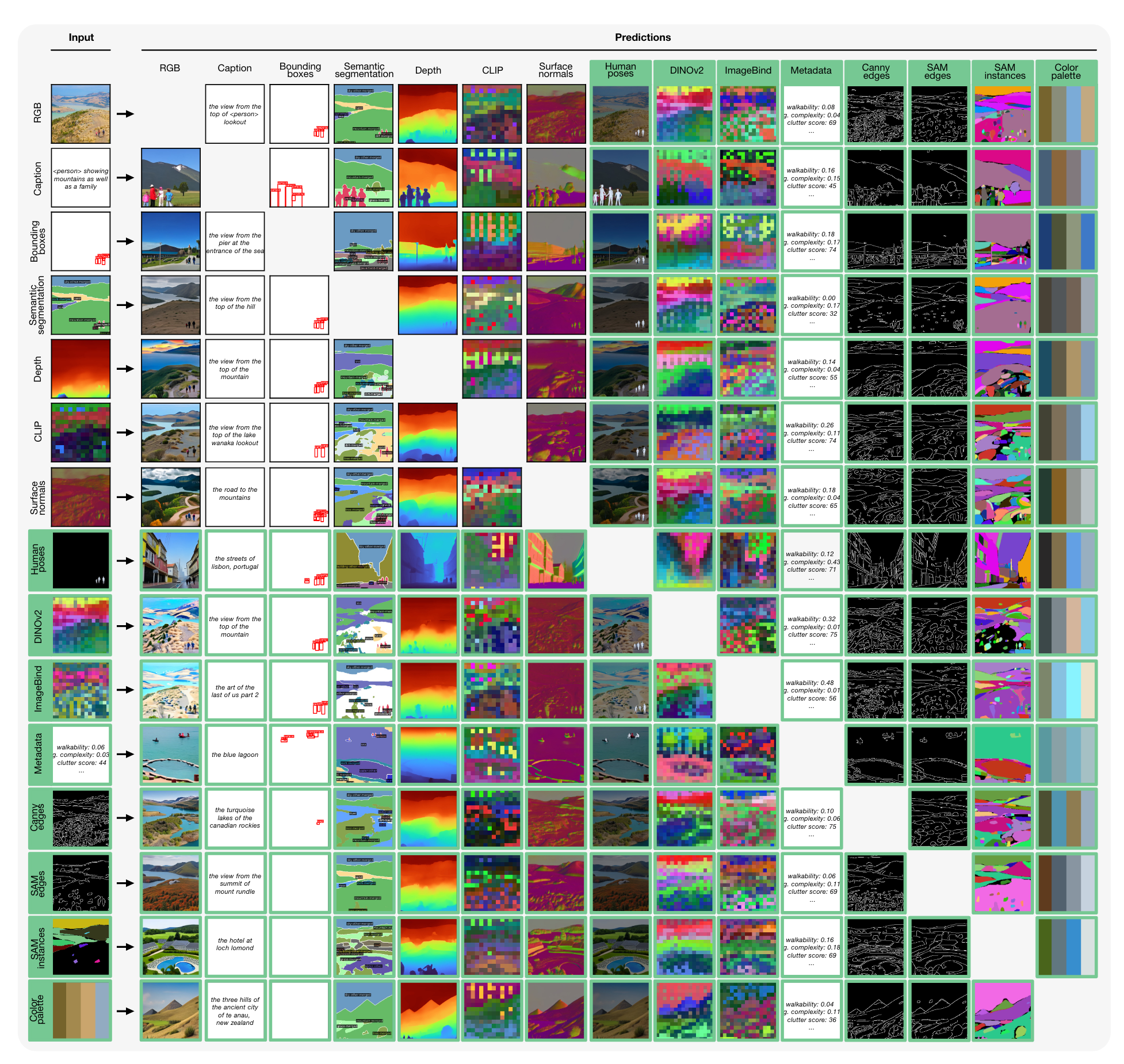
As part of this blog post we will focus more on retrieval rather than generation. But, the basic concepts remain the same.

Note

The authors have open sourced all code here - https://github.com/apple/ml-4m.

As part of this blog post we will focus more on retrieval rather than generation. But, the basic concepts remain the same. With that being said, let’s get started with image retrieval.

2.2 Image retrieval using 4M-21

Figure 4: Different modes of multimodal retrieval

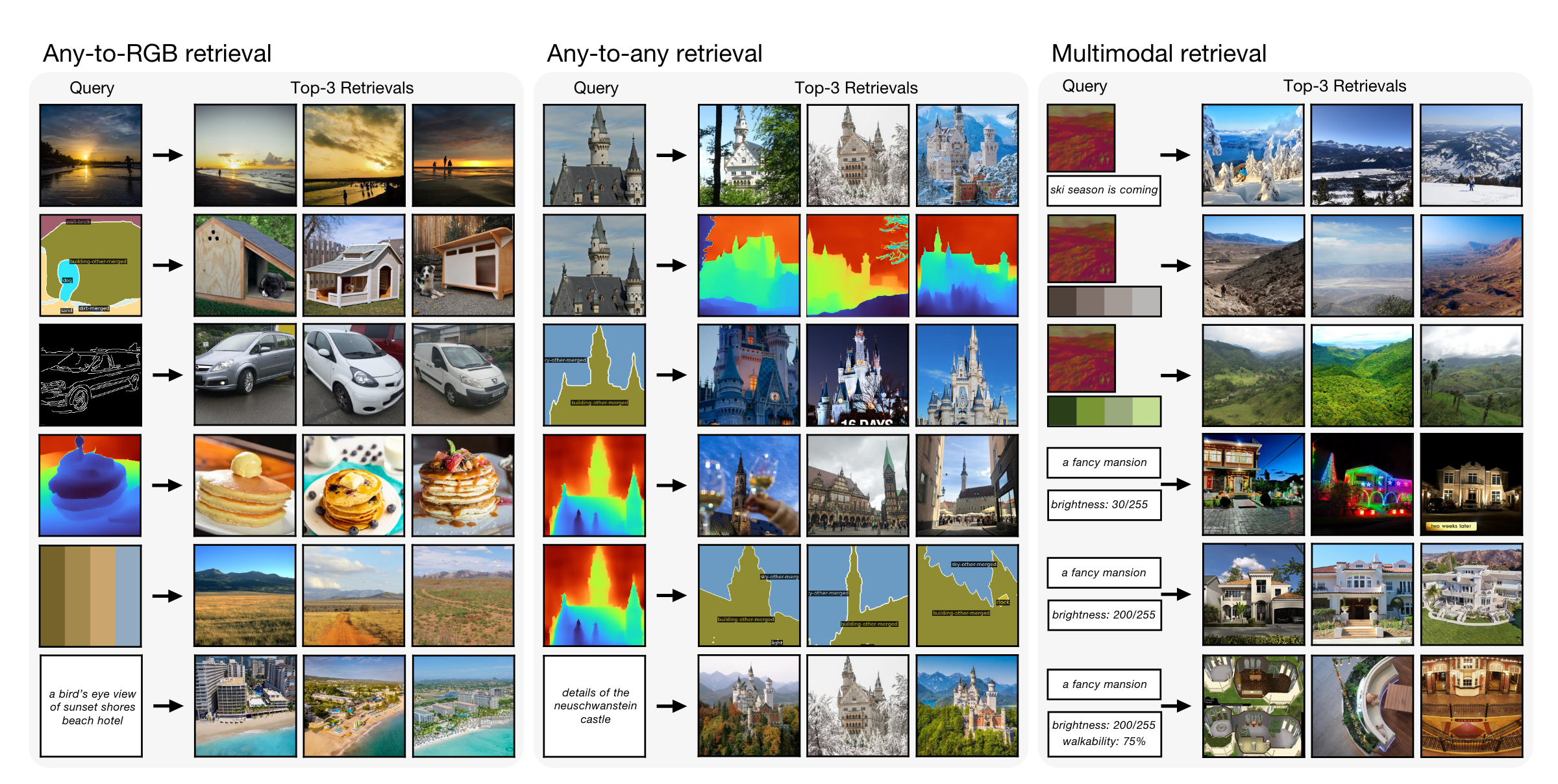
As can be seen above, the authors showcased that the model is capable of using any or subet of 21 modalities as input to retrieve similar images from a database. The query consist of one or more modalities from Figure 2. As part of this blog post, we will be focusing on the “caption + metadata -> RGB” retrieval example.

In Figure 4, given the inputs “a fancy mansion” and “brightness 200/255”, the model was able to return very bright images of a mansion. Doing the same for “brightness 30/255” returns darker images of mansions. We will be replicating this functionality as part of this blog post.

Note

Figure 4 above is what prompted the idea for this blog post. What if we can utilise some or all of the modalities to query our own custom databases?

Thank you dear authors for answering all my questions.

We could have also added any of the input modalities from Figure 4 to our demo but we will leave this to the reader as an exercise to build on top of the code shared in this blog post. We have kept the input modalities limited to two as part of this blog post:

1. Image description (caption)
2. Metadata (such as brightness, number of items per image)

As part of writing this blog post, we did experiment with other modalities such as:

1. Input image (using an image to find similar images)
2. Colour palette (using color palette to find similar images matching the colour schema)

Please refer to Section 2.4 for our findings on our custom database. Using color palette was not giving satisying results. We tried both EPFL-VILAB/4M-21_XL and EPFL-VILAB/4M-21_L models for the same.

Expand to learn more about how to use color-palette and more metadata as inputs to the model

In Section 2.4 we will share with the reader how to extend the app to add color palette as an input the model on top of what has been shared in the demo.

We also showcase to the reader how to extend the app to use other metadata such as:

1. Crowdedness score: number of humans
2. SAM clutter score: number of SAM instances
3. COCO clutter score: number of COCO [55] instances
4. COCO instance diversity: number of unique COCO instance classes
5. Walkability score: % of pixels belonging to walkable COCO semantic classes such as ‘road’
6. Semantic diversity: number of unique COCO semantic classes
7. Caption length: length of the caption in characters, words, and sentences
8. Geometric complexity: angular variance of surface normals
9. Occlusion score: % of occlusion edges over a fixed threshold

Having said that, let’s dig deep into the paper and understand how this model is able to distill information from multiple modalities.

As part of the training, each modality from Figure 2 was encoded using modality specific tokenizers. From the paper:

We employ suitable tokenization schemes for different modalities based on their format and performance. For image-like modalities and feature maps, we use spatial VQ-VAEs with optional diffusion decoders for detail rich modalities like RGB. For non-spatial modalities like global tokens or parameterized poses, we compress them to a fixed number of discrete tokens using Memcodes with MLP encoders and decoders. All sequence modalities are encoded as text using WordPiece.

Figure 5: Tokenization overview

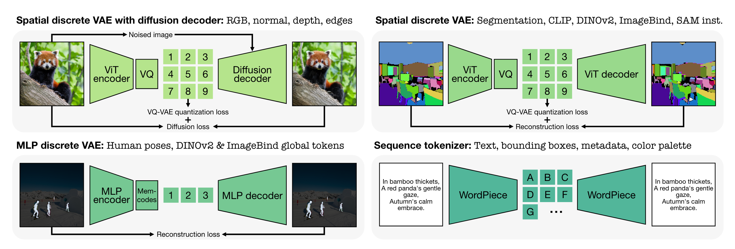
What this means is that authors were able to represent information into a limited number of tokens for multiple modalities. By training modality specific tokenizers, the authors were able to transform different modalities into a common representation. After converting all modalities to a common representation, the authors were able to train a standard encoder-decoder transformer. During training, random subsets of these tokens are selected from all modalities as inputs and targets, and the objective is to predict one subset from the other.

Figure 6: Method overview

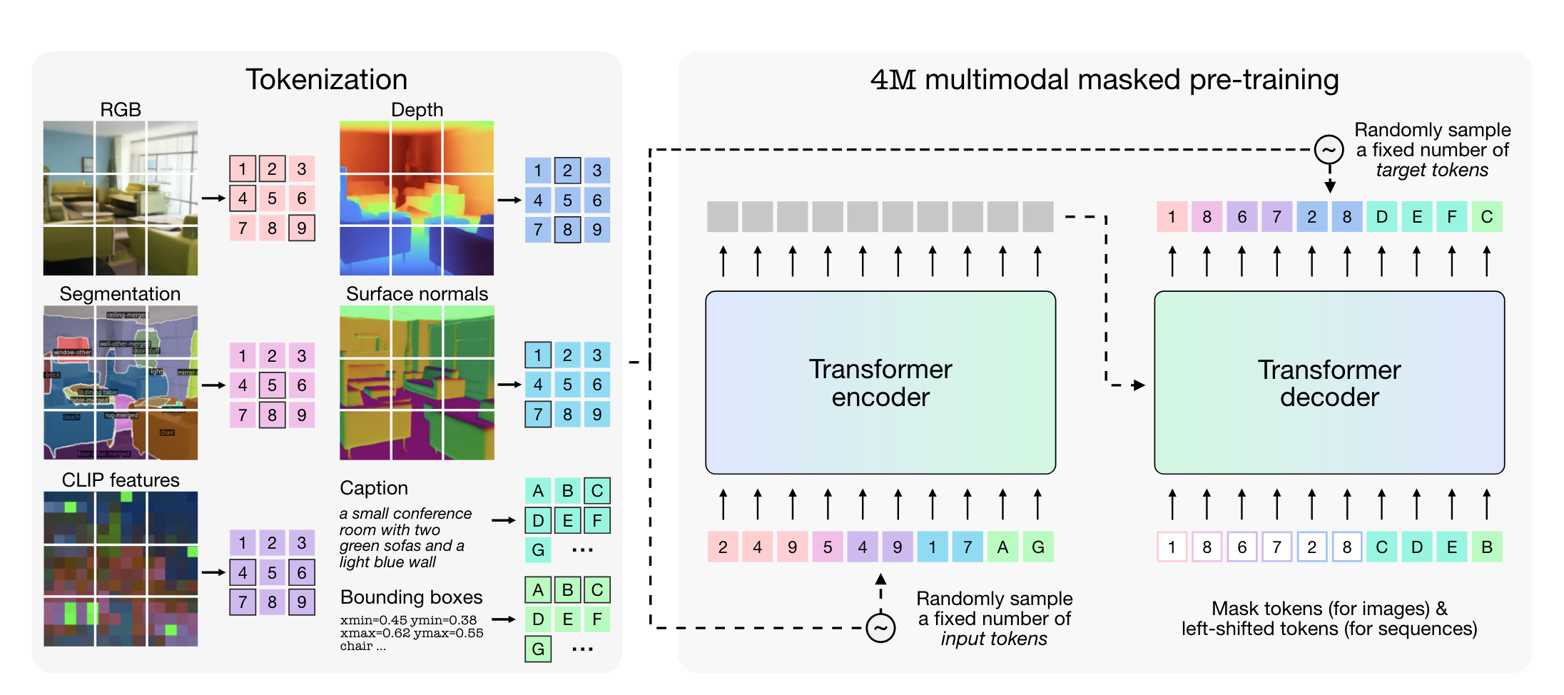
The complete method overview was shared by the authors in the 4M: Massively Multimodal Masked Modeling Mizrahi et al. (2023) paper.

Mizrahi, David, Roman Bachmann, Oğuzhan Fatih Kar, Teresa Yeo, Mingfei Gao, Afshin Dehghan, and Amir Zamir. 2023. “4M: Massively Multimodal Masked Modeling.” https://arxiv.org/abs/2312.06647.

As can be seen, here’s what’s exactly going on:

1. First the different modalities are converted to a number of tokens using modality specific tokenizers
2. A random subset of tokens are selected as input
3. A random subset of tokens are selected as output

By doing so, the model learns to take in all or a subset of input modalities and predicts all or a subset of output modalities thus it is termed an “any-to-any vision model”.

Now that we have a basic understanding of how the model works, let’ start building the retrieval app in Python.

2.3 Python code for image retrieval

We will closely follow the demo notebook shared by the authors and build the retrieval sytem on top of it using a custom database (in this case a sample of 15 images).

As also mentioned in the paper,

Our model can also perform multimodal retrievals by predicting global embeddings of DINOv2 and ImageBind from any (subset) of the input modalities. Once the global embeddings are obtained, the retrieval is done by finding the retrieval set samples with the smallest cosine distance to the query.

We can utilize either Imagebind or Dino-V2 to encode images as embeddings, as part of this demo we utilise DINOv2 global embeddings for retrieval.

ImageBind: One Embedding Space To Bind Them All Girdhar et al. (2023) and DINOv2: Learning Robust Visual Features without Supervision Oquab et al. (2024) are both multi-modal vision models released previously by Meta. They are both capable of representing images to an embedding space. We donot dig deeper into these models as part of this blog post.

Girdhar, Rohit, Alaaeldin El-Nouby, Zhuang Liu, Mannat Singh, Kalyan Vasudev Alwala, Armand Joulin, and Ishan Misra. 2023. “ImageBind: One Embedding Space to Bind Them All.” https://arxiv.org/abs/2305.05665.

Oquab, Maxime, Timothée Darcet, Théo Moutakanni, Huy Vo, Marc Szafraniec, Vasil Khalidov, Pierre Fernandez, et al. 2024. “DINOv2: Learning Robust Visual Features Without Supervision.” https://arxiv.org/abs/2304.07193.

2.3.1 Building the database

Since we wanted to showcase image description, brightness and number of items, our database consists of 15 images downloaded manually using google image search. The complete database can be found - here.

Expand to learn more about creating your own database

Creating your own Huggingface dataset using an image folder is as simple as:

from datasets import load_dataset
dataset = load_dataset("imagefolder", data_dir="path/to/data")
dataset.push_to_hub()

You can read more about it here.

from datasets import load_dataset
dataset = load_dataset("aroraaman/4m-21-demo")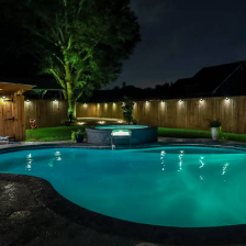
len(dataset['train'])

15

The dataset consists of a mix of dark and bright images of dining room and swimming pool. Some images contain lot of items and are cluttered while others look more “empty”. Images are of type .png, .jpg, .webp we & .jpeg.

dataset['train']['image']

[<PIL.WebPImagePlugin.WebPImageFile image mode=RGB size=852x1200>,
 <PIL.JpegImagePlugin.JpegImageFile image mode=RGB size=1280x853>,
 <PIL.PngImagePlugin.PngImageFile image mode=P size=1500x1284>,
 <PIL.JpegImagePlugin.JpegImageFile image mode=RGB size=564x846>,
 <PIL.JpegImagePlugin.JpegImageFile image mode=RGB size=736x552>,
 <PIL.JpegImagePlugin.JpegImageFile image mode=RGB size=275x183>,
 <PIL.JpegImagePlugin.JpegImageFile image mode=RGB size=300x168>,
 <PIL.JpegImagePlugin.JpegImageFile image mode=RGB size=194x259>,
 <PIL.JpegImagePlugin.JpegImageFile image mode=RGB size=275x183>,
 <PIL.JpegImagePlugin.JpegImageFile image mode=RGB size=616x462>,
 <PIL.JpegImagePlugin.JpegImageFile image mode=RGB size=605x694>,
 <PIL.JpegImagePlugin.JpegImageFile image mode=RGB size=612x408>,
 <PIL.Image.Image image mode=RGB size=635x272>,
 <PIL.WebPImagePlugin.WebPImageFile image mode=RGB size=800x533>,
 <PIL.JpegImagePlugin.JpegImageFile image mode=RGB size=2399x3229>]

Now that we have a list of images that we want to use as our database, let’s use DINOv2 to convert them to embeddings.

from torch.utils.data import Dataset, DataLoader
import torch.nn as nn
from pathlib import Path
import numpy as np
from PIL import Image
import albumentations as A
import torch
from tqdm.notebook import tqdm

Now, let’s load the DINOv2 model as our feature extractor. Speicifically we will be using the ViT-B14 version as mentioned in the Bachmann et al. (2024) paper.

device = "cuda" if torch.cuda.is_available() else "cpu"
feature_extractor = torch.hub.load('facebookresearch/dinov2', 'dinov2_vitb14')
feature_extractor = feature_extractor.to(device)

Using cache found in /home/ubuntu/.cache/torch/hub/facebookresearch_dinov2_main
INFO:dinov2:using MLP layer as FFN

We transform every image by downsizing each image such that the shortest side is of size 224 pixels. We then center crop the image such that all images are of size 224x224. We use Albumentations library Buslaev et al. (2020) for the transforms.

Buslaev, Alexander, Vladimir I. Iglovikov, Eugene Khvedchenya, Alex Parinov, Mikhail Druzhinin, and Alexandr A. Kalinin. 2020. “Albumentations: Fast and Flexible Image Augmentations.” Information 11 (2). https://doi.org/10.3390/info11020125.

class FeatureExtractionDataset(Dataset):
    def __init__(self, feature_extractor: nn.Module, path: str, img_sz=224):
        super().__init__()
        self.feature_extractor=feature_extractor
        self.path = Path(path)
        self.files = list(self.path.rglob("*"))
        self.tfms = A.Compose([
            A.SmallestMaxSize(img_sz),
            A.CenterCrop(img_sz, img_sz)
        ])
        self.device = "cuda" if torch.cuda.is_available() else "cpu"
        
    def __len__(self): return len(self.files)
    
    def __getitem__(self, idx):
        img = Image.open(self.files[idx]).convert("RGB")
        img = np.array(img)
        img = self.tfms(image=img)['image']
        img = torch.tensor(img, dtype=torch.float32)/255.
        img = img.permute(2,0,1)
        return img

Next, we can simply build the dataset, dataloader and store the image embeddings as a PyTorch tensor.

# Create the Dataset
dataset = FeatureExtractionDataset(
    feature_extractor=feature_extractor, 
    path="/path/to/data"
)
# Create the DataLoader
dataloader = DataLoader(
    dataset,
    batch_size=batch_size,  
    shuffle=False,
    num_workers=16,  
    pin_memory=True
)

Finally we can extract the features from each image and store as a PyTorch Tensor.

features = []
for i,batch in tqdm(enumerate(dataloader), total=(len(dataset)//batch_size)+1):
    batch = batch.to(device)
    with torch.no_grad():
        _f = feature_extractor(batch)
    _f = _f.to("cpu")
    features.append(_f)
    
features = torch.concat(features)
torch.save(features, "./image_embeddings.pt")

And that’s it! We have successfully created our image database that we will retrieve similar images from based on a query.

2.3.2 Inference with 4M-21model EPFL-VILAB/4M-21_L to get most similar image

So now that we have the database, our next step is to actually be able to use inputs such as “caption”, “brightness” and “number of items” to get an embedding that will be used as our “query”.

We will closely follow the demo notebook shared by the authors.

import torch
from fourm.models.fm import FM
from fourm.vq.vqvae import VQVAE
from tokenizers import Tokenizer
from fourm.models.generate import (
    GenerationSampler,
    build_chained_generation_schedules,
    init_empty_target_modality,
    custom_text,
)
from fourm.data.modality_info import MODALITY_INFO
from fourm.utils.plotting_utils import decode_dict
from fourm.vq.vqvae import VQVAE

DEVICE = "cuda" if torch.cuda.is_available() else "cpu"
IMG_SIZE = 224
TOKENIZER_PATH = "./fourm/utils/tokenizer/trained/text_tokenizer_4m_wordpiece_30k.json"
FM_MODEL_PATH = "EPFL-VILAB/4M-21_L"
IMAGE_DATASET_PATH = "/home/ubuntu/GIT_REPOS/ml-4m/data/custom_data/"

All tokenizers have been made available on the hub - EPFL VILAB. For our demo, we only need the text tokenizer, since we are using captions and metadata as inputs (both as text). We will also need to the fourm model to create the sampler that is able to create query embedding using input caption & metadata.

text_tokenizer = Tokenizer.from_file(TOKENIZER_PATH)
fm_model = FM.from_pretrained(FM_MODEL_PATH).eval().to(DEVICE)
sampler = GenerationSampler(fm_model)

Below, our input conditional domains are caption & metadata. And our target domain is tok_dinov2_global. As discussed in the paper, we want to obtain the global embeddings of DINOv2 using input modalities for retrieval.

Note

The authors shared how to do multimodal retrieval in code here.

# Generation configurations
cond_domains = ["caption", "metadata"]
target_domains = ["tok_dinov2_global",]
tokens_per_target = [16]
generation_config = {
    "autoregression_schemes": ["roar"],
    "decoding_steps": [1],
    "token_decoding_schedules": ["linear"],
    "temps": [2.0],
    "temp_schedules": ["onex:0.5:0.5"],
    "cfg_scales": [1.0],
    "cfg_schedules": ["constant"],
    "cfg_grow_conditioning": True,
}
top_p, top_k = 0.8, 0.0

schedule = build_chained_generation_schedules(
    cond_domains=cond_domains,
    target_domains=target_domains,
    tokens_per_target=tokens_per_target,
    **generation_config
)

Now that we have a generation schedule to use caption and metadata as inputs to generate target tok_dinov2_global, we can create our dictionary of input and target modalities. let’s initialise the sample.

batched_sample = {}
for target_mod, ntoks in zip(target_domains, tokens_per_target):
    batched_sample = init_empty_target_modality(
        batched_sample, MODALITY_INFO, target_mod, 1, ntoks, DEVICE
    )
    

Let’s say that we want to retrieve a dark image of a swimming pool. So our input caption would be ‘swimming pool’, and metadata is passed in combination of V1 and V0s.

V1 represents which metadata to pass in, the encoding for each metadata type is here.

Brightness is encoded with number 10, and takes in range of values from 0-255. 0 represents a dark image whereas 255 represents a bright image. So to represent a brightness of 50/255, we will write V1=10 V0=50.

caption = "Swimming pool"
metadata = "v1=10 v0=68" #brightness 68/255 as metadata

Let’s create the required dictionaries by the model as input using custom_text method as in the demo notebook.

batched_sample = custom_text(
    batched_sample,
    input_text=caption,
    eos_token="[EOS]",
    key="caption",
    device=DEVICE,
    text_tokenizer=text_tokenizer,
)
batched_sample = custom_text(
    batched_sample,
    input_text=metadata,
    eos_token="[EOS]",
    key="metadata",
    device=DEVICE,
    text_tokenizer=text_tokenizer,
)

Now, we can utilise the sampler that we created before to get the output from our model.

out_dict = sampler.generate(
    batched_sample,
    schedule,
    text_tokenizer=text_tokenizer,
    verbose=True,
    seed=0,
    top_p=top_p,
    top_k=top_k,
)

1it [00:00,  1.20it/s]

This output dictionary consists of tok_dinov2_global as key and the tensor represents the token IDs that make up the representation of the DINOv2 global embeddings.

out_dict['tok_dinov2_global']['tensor']

tensor([[5426, 6424, 5294, 5716,  189, 4065, 7631, 8145, 3108, 7638, 4331, 7005,
         5675, 1472, 3069, 5687]], device='cuda:0')

Let’s now use the decoder to get a 768 representation embedding for the image that becomes our “query” for retrieval purposes. To decode the tokens to the respective embedding, we will need to load the necessary VQ-VAE as well that was used during training.

VQVAE_PATH = "EPFL-VILAB/4M_tokenizers_DINOv2-B14-global_8k_16_224"
vqvae = VQVAE.from_pretrained(VQVAE_PATH)

Let’s now get the image embeddings using decode_dict as in the demo notebook.

with torch.no_grad():
    dec_dict = decode_dict(
        out_dict, {"tok_dinov2_global": vqvae.to(DEVICE)}, text_tokenizer, 
        image_size=IMG_SIZE, patch_size=16, decoding_steps=1
    )

dec_dict["tok_dinov2_global"].shape

torch.Size([768])

As can be seen we have an embedding of size 768 which is our query embedding. Using cosine similarity, we can retrieve the most similar embedding from our image database.

Figure 7: Image retrieval using EPFL-VILAB/4M-21_L for “swimming pool” and 68/255 brightness

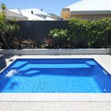
As can be seen, the model sucessfully returns the image of a swimming pool for low brightness. If we increased the brightness to 255/255 we get the following image.

Figure 8: Image retrieval using EPFL-VILAB/4M-21_L for “swimming pool” and 255/255 brightness

2.3.3 Gradio app with required filters

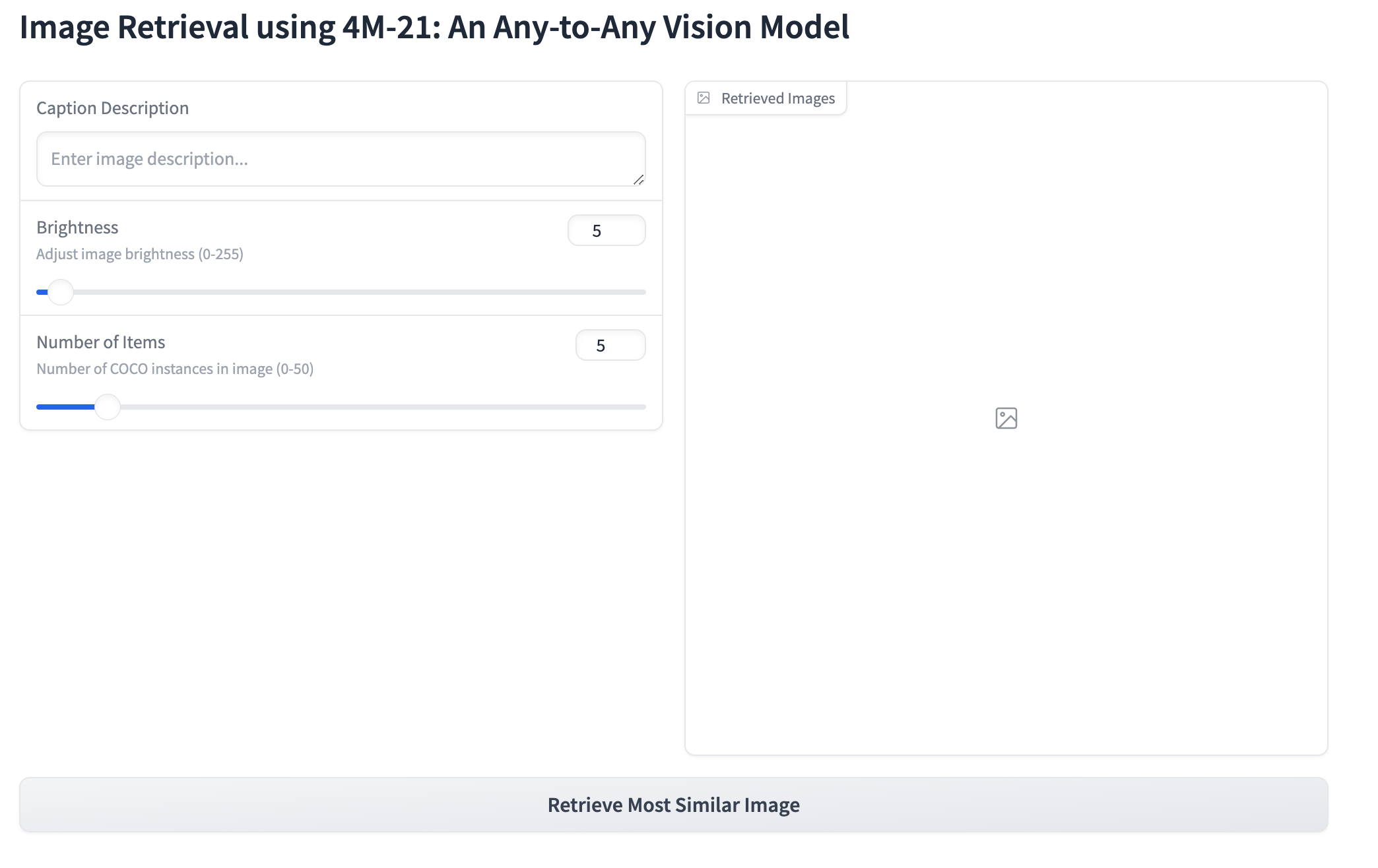
Now that we have all the underlying code, we can simply build a Gradio interface for the same! Why? This makes it very easy for all to use and play with the 4M-21 model. Feel free to create your own apps too. If you do, please don’t forget to let me know about it on my Twitter - https://x.com/amaarora.

The code for the gradio app is pretty simple, I actually used Claude 3.5 Sonnet to help me build the app.

with gr.Blocks() as demo:
    gr.Markdown("# Image Retrieval using 4M-21: An Any-to-Any Vision Model")
    with gr.Row():
        with gr.Column(scale=1):
            caption = gr.Textbox(
                label="Caption Description", placeholder="Enter image description..."
            )
            brightness = gr.Slider(
                minimum=0, maximum=255, value=5, step=1, 
                label="Brightness", info="Adjust image brightness (0-255)"
            )
            num_items = gr.Slider(
                minimum=0, maximum=50, value=5, step=1, 
                label="Number of Items", info="Number of COCO instances in image (0-50)"
            )
        with gr.Column(scale=1):
            output_images = gr.Gallery(
                label="Retrieved Images",
                show_label=True,
                elem_id="gallery",
                columns=2,
                rows=2,
                height=512,
            )
    submit_btn = gr.Button("Retrieve Most Similar Image")
    submit_btn.click(
        fn=get_similar_images,
        inputs=[caption, brightness, num_items],
        outputs=output_images,
    )

Using above code, allows us to create the Gradio app that was shared in Figure 1.

Figure 9: caption & metadata retrieval using EPFL-VILAB/4M-21_L

2.3.4 Deploy app to HuggingFace hub

We have deployed the app sucessfully to huggingface Spaces. We followed the documentation here.

You can find the huggingface space here.

Somem minor changes that we had to do between local and for the app to deployed on huggingface spaces:

1. All binary files had to be tracked by git-lfs. Read more about it here
2. Convert dataset to a huggingface dataset, as we were not able to upload .jpg, .png or other files
3. The complete source code for the gradio app that works on HF spaces can be found here.

Overall it was pretty straightforward and easy to deploy!

2.4 Appendix A

We used EPFL-VILAB/4M-21_L for all our experiments and image retrieval due to memory constraints. We found EPFL-VILAB/4M-21_XL requires around 28GB of VRAM along with respective tokenizers, and runtimes were slow on a A100 40GB instance.

Figure 10: rgb-to-any retrieval using EPFL-VILAB/4M-21_L

2.4.1 Adding color palette as inputs

From the paper:

For every RGB image, we extract between one and seven color palettes using PyPalette. During training, we randomly sample one of the color palettes to enable users to input palettes with different levels of granularity.

color palette sequence is formed as color = c R = r G = g B = b R = r, … where c takes a value between 1 and 7 and specifies the number of colors in the palette and r, g, b takes values between 0-255.

We can write a small python function to convert any of seaborn color palettes to the required format. Also, as per the color palette transform, the tokenizer expexts “color” to be replaced by “v1” and r,g,b with “v0”.

Therefore, a color palette represented by color=1 r=166 g=206 b=227 should be transformed to v1=1 v0=166 v0=206 v0=227.

import seaborn as sns

def generate_color_palette(num_colors=2, palette_name="Paired"):
    palette = sns.color_palette(palette_name, num_colors)
    rgb_values = [(int(r*255), int(g*255), int(b*255)) for r, g, b in palette]
    color_strings = [f"v0={r} v0={g} v0={b}" for r, g, b in rgb_values]
    color_palette = f"v1={num_colors} " + " ".join(color_strings)
    return palette, color_palette

palette, color_palette_string = generate_color_palette(num_colors=2)
palette

color_palette_string

'v1=2 v0=166 v0=206 v0=227 v0=31 v0=120 v0=180'

Now we can simply pass in the string above as input and use custom_text function on our batched_sample to prepare batch for input to the model. We also need to add color_palette to the conditional domain as input.

cond_domains = ["caption", "metadata", "color_palette"]

Once that’s done, we can now take our color_palette_string as input and created the batched_sample as before in Section 2.3.2.

batched_sample = custom_text(
    batched_sample,
    input_text=caption,
    eos_token="[EOS]",
    key="caption",
    device=DEVICE,
    text_tokenizer=text_tokenizer,
)

And that’s it! Everything else remains the same!

2.4.2 Adding more metadata as input

In the demo application, we only utilised brightness and number of items as metadata inputs. But as descriped in the paper, we could have used many more metadata as inputs.

To pass in any of the metadata available here, just pass in v1=[key] v0=[val] to the input string.

For example, to add in metadata: “brightness 50/255 contrast 50/127 walkability 25/50”, simply write it as:

v1=10 v0=50 v1=11 v0=50 v1=14 v0=25

We simply replace the words by their corresponding metadata key and add the value with v0=[val].

And that’s it! Now the reader can also add any of the 20 metadata filters that the authors have trained the 4M-21 model on.

2.5 Conclusion

As part of this blog post, we looked into the 4M-21: An Any-to-Any Vision Model for Tens of Tasks and Modalities Bachmann et al. (2024) paper and built an image retriever app on top as a real world application.

Bachmann, Roman, Oğuzhan Fatih Kar, David Mizrahi, Ali Garjani, Mingfei Gao, David Griffiths, Jiaming Hu, Afshin Dehghan, and Amir Zamir. 2024. “4M-21: An Any-to-Any Vision Model for Tens of Tasks and Modalities.” https://arxiv.org/abs/2406.09406.

In Section 2.3, we also looked at the Python code to be able to build such an app on any custom database. We built a gradio app for demo purpose and also deployed it to Huggingface Spaces!

All code and corresponding files can be found here.

Finally in Section 2.4, we looked at ways of extending the demo and adding color palettes and more metadata as input filters for retrieval!

Thank you readers for your time. If you have any feedback, please feel free to share it with me here.

Subscribe to Aman Arora's blog:

* indicates required

Email Address *